Stable Diffusion - the current state of the art
At this point most of the Internet users have at least seen the spectacular images outputted by the breakthrough generative models from the last few years. Midjourney, DALLE-3, NovelAI and Stable Diffusion are just a few of the many services available at the moment. They all work in a similar manner - you, the user, provide a text prompt that guides the model in the generation process. It outputs an image in the size of your choosing. On the surface, that’s all you need to generate your art.
When you dig under the hood, you’re going to discover some advanced options to tweak. Playing around with them can lead to drastically improved results. But how do you use them properly, if their names don’t really describe what they control? Steps, guidance, image to image - what is this and where did it come from? You’re about to find out in this tutorial.
Understanding those features requires us to dive deeper into the inner workings of generative AI. It’s a difficult subject, considering that Midjourney, NovelAI and DALLE-3 are all proprietary tech. Stable Diffusion is not, though. We don’t know how propietary ones work in depth - but the advanced options they offer sure are strikingly similar to the open source Stable Diffusion. That’s why this open source tool is great for understanding text to image generation in general.
How humans do it
Biology and natural evolution has inspired many human discoveries. So, it’s probably not a bad idea to first look at how a trained human brain would approach the whole “art” problem.
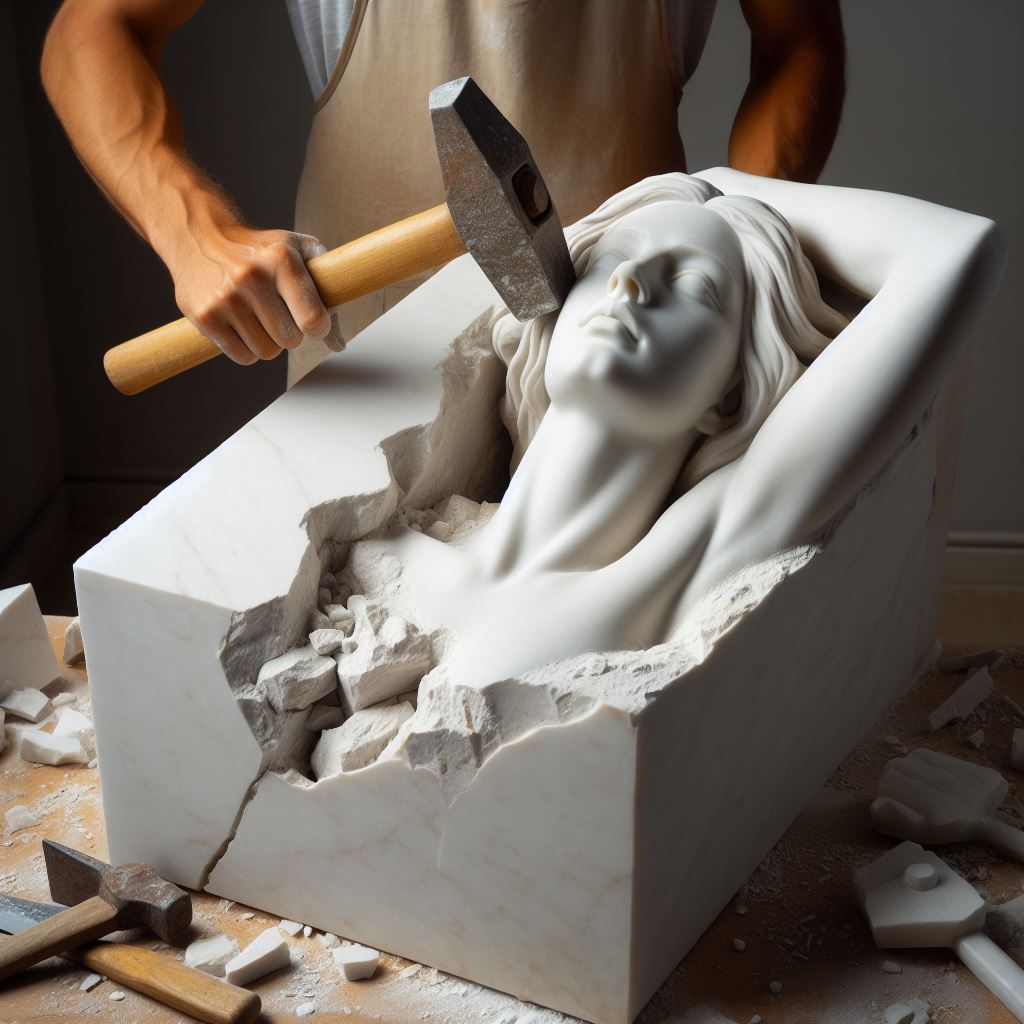
You might have seen human artists at work. Whether they’re painters, designers or sculptors, they all share a similar approach to creating their art pieces. It’s a gradual process. They start off from a solid block of material (or an empty canvas). Initially, they try to find general shapes and silhouettes of their piece. Only once those are set, do they move to adding in finer details and correcting any defects.
The tensor operations we’re going to look at can be intimidating at first. So, it’s good to keep in mind the human approach. Although it’s not 100% mirrored, we’ll be trying to achieve a process that resembles the professional artists’ workflow.
There and back again - the diffusion model
Noise predictor
Although the process of converting a text prompt into an image is a little bit more complicated than that, at the heart of it lies the noise predictor model (we’re going to cover the rest afterward).
It’s a deep learning model revolving around a very clever idea. Suppose you have a set of images of different vehicles: cars, trains, boats and planes. You would go ahead and add some random noise to the images. Then take those pictures and corrupt them again, and again. In the end it would reduce them to an unrecognizable set of pixels. Side by side, the comparison of before vs after multiple corruption steps would look like this:
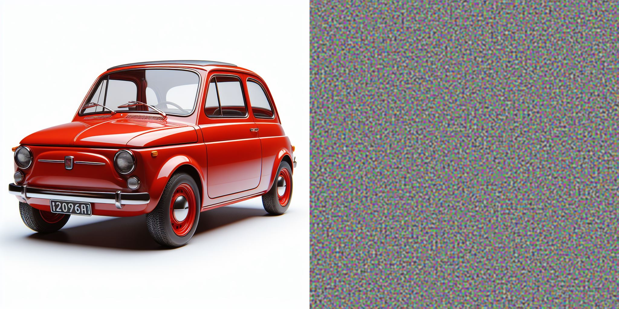
At this point you would have a dataset of images, corrupted to a varied degree. Then you would feed the noised image, along with its vehicle category (in the case above, “car”) into the model. Its task would be to predict a tensor representing the noise that was added to the original image. In case you’re wondering, in this case of machine learning problem we have a ground truth for our observations (the clean image), so it’s an example of supervised learning.
Let’s assume we’ve successfully trained the model. We could use it to predict the noise that we’ve originally added to the image. After subtracting the predicted noise from the noisy image, we would get the original one. Great, now we can fix what we’ve broken in the first place. But, is that the model’s only usage?
Now imagine a situation where we generate a completely new, random, noisy image that was not originally a valid one. Just a bunch of random, gibberish pixels. Then we would feed it to our trained model along with the “plane” label. What would the net do then? Exactly what it was trained to do - predict the noise that was added to the original plane picture. Of course, there was no plane to begin with, but the net will try to recover one anyway. And this way, after subtracting the predicted noise, we will get a completely new, original image of a plane.
It feels like cheating, but that’s actually how diffusion models work. The diffusion part actually refers to the process of corrupting an image with noise. In this regard our way of constructing a training dataset can be referred to as forward diffusion. What we actually want to use though is the reverse diffusion - the process of denoising a gibberish image to recover a clean one.
Step by step
We’ve mentioned real life artists and their stepwise approach to creating an art piece. Turns out this method works quite well for deep learning approach, too.
Our noise predictor gives us a tensor with the predicted noise that we should subtract from the image. If we substract it, in theory, we should get our ready output picture. In practice though, our predictor might not be good enough to clear all the noise from the input gibberish it gets in one go. It’s probably going to do a good job at determining basic shapes, but not finer details. However, if we were to grab what it spits out and feed it as an input to the model again, it could now focus on the finer aspects of the piece.
Let’s remember that the image generation works by removing the noise from an input. If we were to just repeat the process as-is, the model would quickly run out of noise to work with. That’s why, at each time step we will be adding some new noise to the image before processing it by the model. Doing that additionally helps the model deal with difficult generations, as it can get stuck on certain cases. The multi-step approach with gradual adding of the noise tends to produce good and reliable results. Now you know where the name Stable Diffusion came from.
We can repeat the denoising step many, many times. It’s worth remembering though, that the detailing part of the art piece requires more subtlety than the first, crude approach, which only determines the basic shapes and figures. That’s where a parameter called scheduler comes in.

Source: https://iway.org/stable-diffusion-samplers/
It is a value that determines the amount of noise that will be added to the image at a particular step. It tends to decrease with time, since we can expect that the further we go, the more the model will work on the details of our image and not general shapes. As such, it won’t need as much “ammunition” (in the form of noise) to recover them. There are multiple versions of the scheduler, for instance some can decrease the added noise linearly, others (like the scheduler above) exponentially.
I’ve mentioned steps - yes, that’s exactly the “steps” parameter you can see in the services I mentioned at the beginning. For instance, NovelAI allows you to adjust how many steps you wish to dedicate to creating your piece. More steps generally means better results. The model will usually converge on some n step and stop majorly modifying the image further, though. No point in going too crazy, then. Especially given that more steps means more time and precious compute time needed for the generation. Knowing that, you surely understand why adding additional steps usually means paying with your precious subscription tokens.
From diffusion to Stable Diffusion
Latent space diffusion
We’ve just talked about diffusion. It let’s us create completely new images with a clever trick - but we wanted to learn about Stable Diffusion. So, what sets apart the discussed process from one of the current state of the art models?
The answer is, efficiency. For every image in color the number of values you will need your model to generate will be given by:
\[\text{n} = w * h * c\]Where:
- n - the number of values your final image will have
- w - width of the image
- h - height of the image
- c - number of channels; for RGB image (in color) it’s equal to 3 for red, green and blue channels
Imagine generating a 720p portait (1280 x 720) in color - that’s 2764800 values. Let’s size it down to a more modest 512 x 512 - that’s still close to a million (786432) values! That is a lot and even the most modern GPUs will take their time with it. Stable Diffusion was designed with efficiency in mind, to exact this particular problem.
The general idea behind it is: let’s take the original input image and compress it down to a smaller size. Let’s generate a similarly compressed output and only then let’s decompress it to our desired size. We usually refer to compressed images as images in latent space.In practice, for 512 x 512 input, we’re talking 4 x 64 x 64, a standard size for the latent space in Stable Diffusion. If you compare the original 512 x 512 image versus the compressed one, we’re talking 48 times reduction in compute!
This approach would let us save a lot of precious GPU workfload, but wait, can we really do that? Can we just compress an image to some small size, with 4 channels no less and not lose information? It turns out we can, or at least not lose much. But we need a smart way to do that.
Variational Autoencoder
The compression and decompression is handled by the Variational Autoencoder (VAE) neural network. It’s composed of two components, the encoder and decoder. The encoder is responsible for the compression of the input image, while the decoder - for the decompression of the output. Those same components are employed during training (for instance the random noise tensor is added to an already compressed image). It sheds a new light at how the steps we’ve just discussed really work.
The VAE net does not perform magecraft, of course. The reason why it is possible to represent an image in latent space effectively is due to its nature. It is heavily influenced by proximity and regularity. If you grab an image and reduce it a small size, you’re going to lose quality - but you’ll still be able to recognize what the image represents. So even a heavy handed downsizing approach works quite well and shows just how regular images are. The VAE we’re using learns how to additionally squeeze in as much details into the representation so that the loss of information is minimal.
Handling the prompt
What are we missing?
Let’s take a step back and think of how we’ve originally described the training process. The noise predictor, as one of the inputs, would take the type of vehicle as a hint of what should be in the image. This, of course, can be compared to a very simple text prompt that you give from user side in image creation. But, if you’ve ever tried it out, you would know that the service offers you great flexibility. You can pass in a long, complex prompt and the model still interprets it fine, giving you an image beyond a simple “car” or “plane”. How does it happen?
From text to tokens, and to embeddings
The way Stable Diffusion handles the text prompt (both during training and inference) is based on tokenizing it and converting it to embeddings, which are consumed by the noise prediction model as input.
Tokens are just little pieces of the prompt and can be thought of as the model’s vocabulary. For a start you can think of them as single words of the prompt, but in reality tokens are more complicated than that. They don’t always represent a single word (although they still may). There are also instances where interpunction like whitespace is affixed as part of a token. This makes them more robust than simple words. There are also a lot of different techniques to tokenizing, which produces a whole pletora of different token vocabularies. Stable Diffusion in particular uses CLIP tokenizer. We will come back to it later, when we summarise the entire pipeline. No matter the technique though, the tokens are a result of splitting your prompt into simpler pieces.
Embeddings are learnable vectors. A lot could be said about them, but if you’re not already familiar, it is a way of providing the model with additional information on the tokens. For instance, as input, we could give the model two numbers - 34 and 555, representing indices of tokens “car” and “audi”. That’s fine, but it would be helpful for the model to know that “audi” and “car” are very similar to each other. Otherwise it sees no particular connection between the two classes. We’re feeding it just two rough numbers, after all. But if we were to give it two vectors, similar to each other in many ways and differing in minor details, it would provide the model with information, that those two tokens deal with similar concepts. In Stable Diffusion we reuse the already learned embeddings (by importing them), which represent the relationships between the tokens. We do not train them ourselves.
So, after we tokenize the prompt into n tokens, and change them into corresponding embeddings, each of length m (all embeddings are equal in length), we get a n x m tensor. This tensor is what we actually feed into the noise predictor as an input.
Guidance
One of the more striking options to choose from in image generation is the guidance. It’s a parameter that lets us control how much freedom the model will have in generating the image and how much will it have to rely on our prompt. Guidance is a major factor in the equation defining the final output of our noise predictor model:
\[∇x log p_γ(x|y) = (1 - γ) ∇x log p(x) + γ ∇x log p(y|x)\]Where:
- ∇x log p(x) - output of the conditional model
- ∇x log p(y|x) - output of the unconditional model
- γ - guidance; on the scale from 0 to 1
If math is not your thing, it can be understood as such:
\[\text{Combined Output} = (1 - γ) * \text{Unconditioned Output} + γ * \text{Conditioned Output}\]In other words, we generate the output of the model two times: first, where we don’t give it any prompt at all (the unconditioned output) and second, where we give it our prompt (the conditioned output). The final, combined output of the model is a proportion of the two. The higher the guidance, the more of the conditioned output will be present in the combined output, up to 100% if we pick guidance equal to 1.
I don’t recommend going too crazy with the guidance, though - leaving the model some room for creativity usually improves the output quality and choking it can lead to weird generations.
This particular form of guidance we’ve just explained is called Classifier-free guidance (CFG). As you may expect, there is also a Classifier guidance, an older approach. It used a trained classifier neural net which took in the n x m prompt embedding tensor and outputted a vector with token “importance” scores. The guidance then decided how much influence those scores will have on the generation. Training a separate classifier was problematic though. The CFG approach is now popular due to simplicity and similar effects.
Putting it all together
Stable Diffusion model pipeline
 Source: https://towardsdatascience.com/stable-diffusion-using-hugging-face-501d8dbdd8
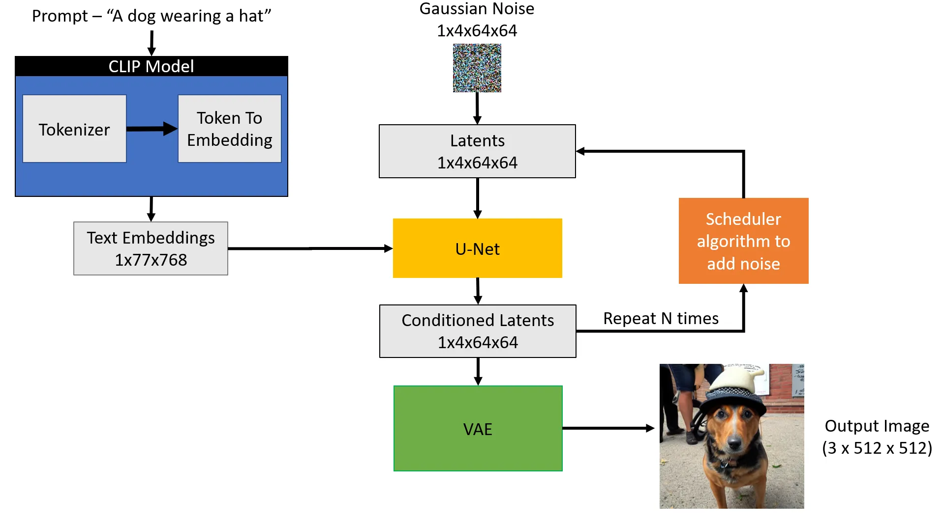
Let’s put it all together, based on the example given above. We want to generate “A dog wearing a hat” and that’t exactly a prompt we provide to the Stable Diffusion model. We press “Go”…and what happens?
Our prompt is first coverted to 77 tokens by the CLIP tokenizer, which are then replaced by their associated embeddings, each of length equal to 768. This gives us the 77 x 768 matrix as our first user-submitted input.
As second input, from Gaussian distribution we generate a tensor in latent space (so of sizes 1 x 4 x 64 x 64). This way we can skip the compression step, which was necessary only during training, where we had to compress our labeled images. This latent space is now random gibberish, but will soon become our output image. In case you’re wondering about the 4-dimensional tensor we’re creating - our noise predictor is able to work with multiple images at the same time. This means we can stack them together as a new dimension (in this case we have only one image, so its value is 1). In other words, our tensor represents: image indices x channels x height x width.
The two input matrices are supplied to the noise predictor (U-Net), generating a 1 x 4 x 64 x 64 output (conditioned output). Then, we produce one more such output, but this time input only the image matrix. This is our unconditioned output. Now we calculate combined output according to our guidance. In the picture those two runs are not separated, so don’t get confused.
Our combined output represents the noise predicted by the model. All we have to do is remove it from the image in a simple subtraction of two tensors. Now that we’ve denoised our image, we’re done with step 1. We want to reach step n, depending on our parameter choice in the beginning.
For step 2 we generate a 1 x 4 x 64 x 64 Gaussian noise tensor according to the algorithm of our scheduler. Then we add it to the image outputted from step 1. As mentioned earlier, this is to help the model get unstuck if it has troubles during generation and supply it with fresh noise to work with. Then, we just follow through the whole process described in step 1.
When the image is done, we need to decompress it. We feed our 1 x 4 x 64 x 64 tensor into the decoder of VAE. We get a single, 3-channeled (colored) dog picture of a dog wearing a hat, so a 1 x 3 x 512 x 512 tensor. Congrats - we’re done!
Image to image
As a final note, let’s quickly discuss the image to image feature of Stable Diffusion, where you supply an existing image, which will be modified according to the given prompt. How does it work? Is there some special method to only modify existing images and not create ones from scratch?
Nope. It’s practically identical to generating them from scratch. Instead of generating a random tensor with gibberish, you take the input picture, compress it to latent space and then corrupt it with noise. The more you corrupt it, the more changed it will come out. A scalar value of magnitude let’s you control how much noise you want to add exactly. The U-Net will then take the picture and denoise it according to the prompt. And (assuming you haven’t completely reduced the picture to just gibberish noise) there will still be traces of your original image left in the noised picture. So the U-Net will just work with it, recovering a picture similar to what you had originally, but with desired changes applied.